We used computer vision to detect and track two seperate Thymios, and switch their positions using following an optimal path, all while avoiding local obstacles.

• Date: December 2019
• Author: Shadi Naguib, Raphael Ausilio, Valentin Karam, Niccolò Stefanini
• Field of Study: Robotics, Navigation, Path Planning, Computer Vision, Filtering
• Context: EPFL Ma-1 Mobile Robotics Project

Goal

We had a lot of freedom in the creation of this project, with our only instructions being to use the Thymio robot and to create a project that included the following four concepts:

• vision
• global navigation
• local navigation
• filtering

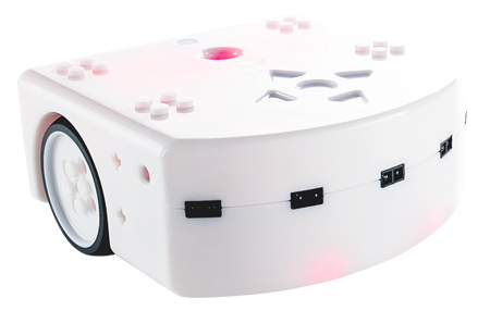
We decided to use two thymio robots in flat arena with stationary global obstacles. The goal was to switch their positions using an optimal path planning algorithm around the global map. Local obstacles were allowed to be introduced into the arena at any moment so we used a collision avoidance algorithm to contour each local obstacle. We used a Kalman filter for position state estimation and correction, using odometry and camera data.

We run a loop based on a finite state machine that stops once each of the two Thymios have reached their goal positions. The robot moves along it’s optimal trajectory, but for each loop it checks for local obstacles with its proximity sensors, and uses the kalmann filter to either correct the deviation from the path, or recalculate a trajectory every 5 loops. If an obstacle is detected, the robot changes state and switches to wall following mode, where it avoids the local obstacle and recalculates an optimal trajectory once avoided.

Vision

We used an external webcam to take a birds eye image of our global map containing the global obstacles and the two Thymios:

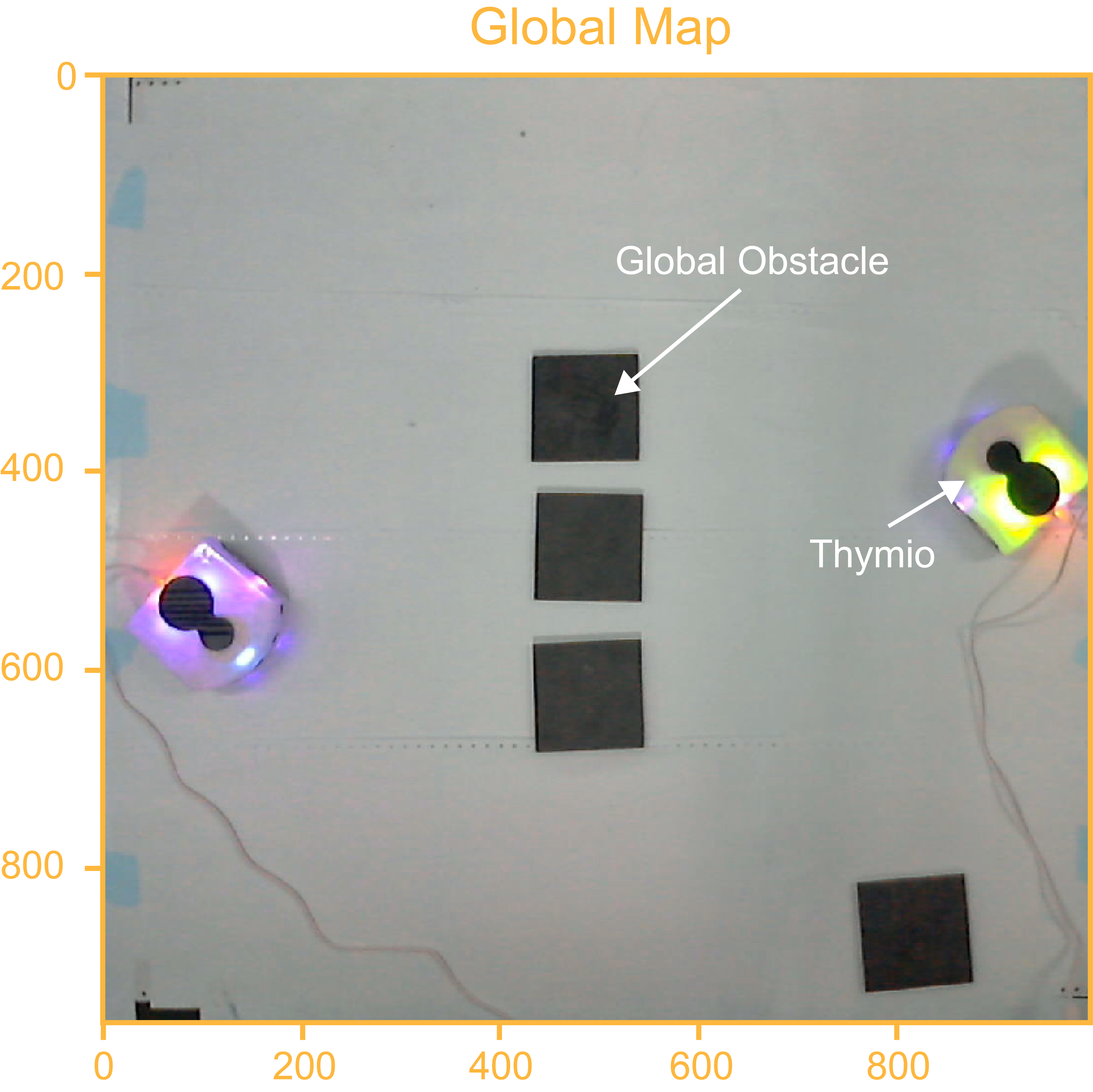
Every time step we take a picture of the global map and filter the image. We use morphological operators that recognize a 3D printed part place on the robot to estimate it’s position and orientation. These operators also detect the global obstacles as shown in the image below. From this we can extract an occupancy grid with the pose of each thymio and obstacle.

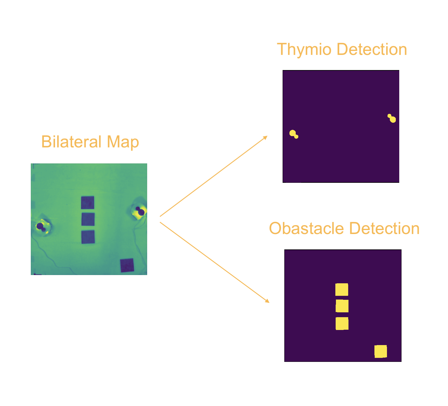
Global Navigation

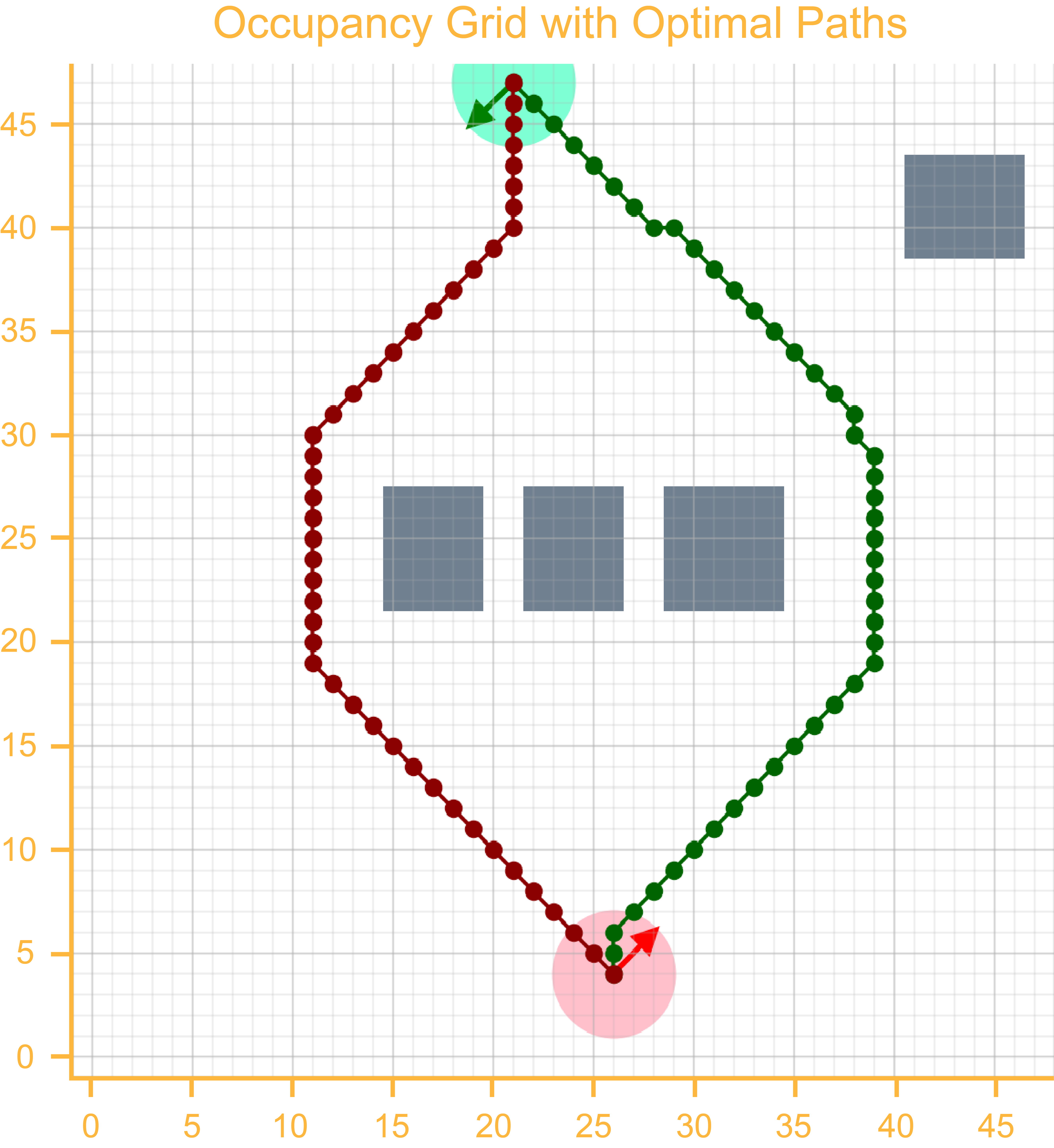
We chose the A* search algorithm thanks to its completeness, optimality, and efficiency. Since the two robots are to switch positions, their optimal paths should theoretically be identical. Therefore we calculate the trajectory for one robot, and consider it to be an obstacle in it’s “half way” position during the calculations for the second robot. This gives us a different path for each robot, which we can plot in the occupancy grid as shown here:

Here we create the different parameters we are going to use for navigation:

• posArray: an array of global path positions [ [x y orientation] … [x y orientation] ]
• movArray: an array of movements for the global path [ [dx dy] … [dx dy] ]
• dirArray: an array of next directions (relative to the robot’s current position) for the global path [d d … d]

The orientation and next directions are defined as follows and are stored as commands for the robot:

Local Navigation

We use the proximity sensors on the thymio robot to check for obstacles during each loop of the algorithm. If a local obstacle is detected, we initiate a wall following (or contouring) algorithm in three parts as follows:

The avoidance is done in three parts and is illustrated in the figure below:

1. Obstacle detected. Approach wall and left or right
2. Left or right wall following
3. If angle error is lower than a threshold value, recalculate optimal trajectory and switch to navigation state

During this time, we force values onto the sensors where the global obstacles are situated to avoid collisions with these.

Filtering

For filtering, we used a Kalman filter. We assume thta the system respects a constant velocity model where the velocity is in cells/degrees per motion. We use the Kalman filter to reestimate the position and a possible correction factor for the position. To filter using the camera detection data, we project the system with a matrix that is an identity for the three first values of the 2D pose [x y orientation]. After tuning we define the variances values for the state and measurement errors. In our case, the camera is supposed to be more trustful than the imprecise odometry, so we give more importance to its estimation.

Every five loops of the algorithm, we apply corrections to the robot’s pose if it has deviated from its trajectory. If the deviation is larger than a user defined threshold, we instruct the algorithm to recalculate a new trajectory using A*.

Additional Material

For any more information on the project, please don’t hesitate to contact me here, or check out the jupyter notebook below.